EPPS Math and Coding Camp
algebra,arithmetic and trig
Instructor: Jonathan Kaufman

2.1 ALgebraic operations
- PEMDAS is the order of operations for all mathematics, starting with whatever is inside the parentheses or brackets \((\cdot), [\cdot]\), then any exponents \((\cdot)^n\), then multiplication and division, and finally addition and subtraction.
- not following PEMDAS will yield incorrect answers fro example \(9+7\times8 +2^2+3\times0\) is different then \(9+(7\times8+2)^2 +(3\times0)\) which is different from \((9+7)\times(8+2^2+3)\times0\)
Ratios, Proportions, and Percentages
- The ratio of two quantities is one divided by the other \(\frac{x}{y}\) is the ratio of x to y. Ratios are also written as \(x:y\).
- Though a ratio may be negative, we typically consider ratio variables that range from \(0\) to \(\infty\).
- The proportion of two variables, on the other hand, is the amount one variable represents of the sum of itself and a second variable: \(|\frac{x}{x+y}|\). A proportion ranges from a minimum of \(0\) to a maximum of \(1\).
- in social science we sommonly focus on proportions such as the proportion of voters, or proportion of a budget and how it is used.
- The percentage one variable represents of a total is the proportion represented over the range from \(0\) to \(100\): \(|\frac{x}{x+y}| \times 100 \%\).
2.2 FUNCTIONS
- A relation that assigns one element of the range to each element of the domain is a function.
- One that assigns a subset of the range to each element of the domain is a correspondence.
2.2.1 Equations
- implicit notation \[ y=f(x) \]
- explicit notation
Example: \(y=3x\)
\(y\) is a function of \(x\);
\(x\) is the argument of the function
2.2.2 Graphs
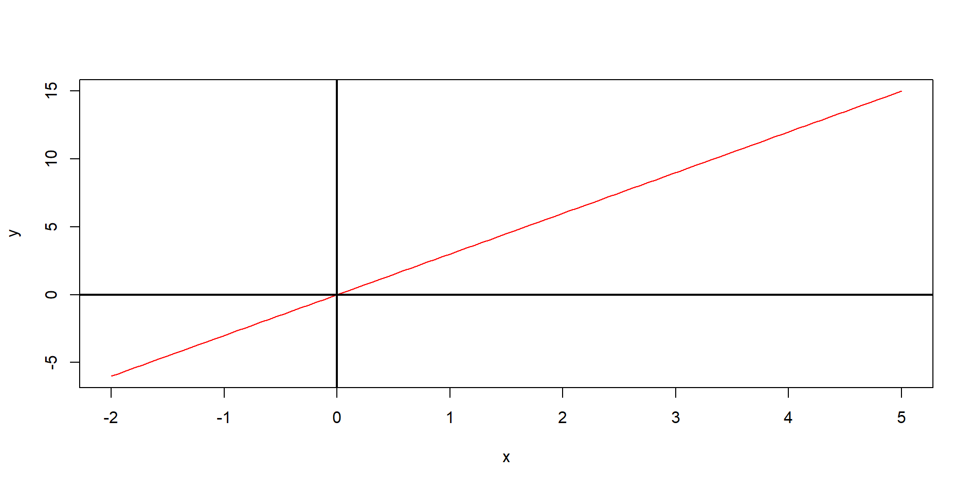
- graph of \(y = 3x\)
2.2.3 Some Properties of Functions
- We define the function \(f\) as \(f(x) : A \rightarrow B\). This is often read as “\(f\) maps \(A\) into \(B\).” \(A\) here is the domain of the function, \(B\) is known as the codomain.
- The set of all values actually reached by running each \(x \in A\) through \(f\) is known as the image, or range, and it is necessarily a subset of B.
- function composition: \(g \circ f(x)\) or \(g(f(x))\)
2.2.3 Function Composition
- \(g \circ f(x) = g(f(x))\) is read as g of f of x
- Example:
- if \(f(n) = 2n , g(n) = n^3\)
- then \(g(f(n)) = (2n)^3 = 8n^3\)
- and \(f(g(n)) = 2(n^3) = 2n^3\)
- Hence \(g(f(n)) \neq f(g(n)))\).
Types of Functions
Surjective (Onto)
- Every value in the codomain is produced by some value in the domain.
Injective (One-to-One)
- Each value in the range comes from only one value in the domain.
Bijective
- Both injective and surjective → function is invertible.
2.2.3.1 Identity and Inverse Functions
Identity Function
- Where both domain and co-domain are identical. It maps elements to themselves. \(f(x) = x, f(x): A \rightarrow A\)
| Term | Meaning |
|---|---|
| Identity function | Elements in domain are mapped to identical elements in codomain |
| Inverse function | Function that when composed with original function returns identity function |
| Surjective (onto) | Every value in codomain produced by value in domain |
| Injective (one-to-one) | Each value in range comes from only one value in domain |
| Bijective (invertible) | Both surjective and injective; function has an inverse |
Monotonic Functions
- Increasing: A function is increasing on interval I if \[ f(b)\geq f(a)\ when\ b > a\ where\ a,b \in I \]
- Strictly Increasing: \[ f(b) > f(a) \ when\ b > a\ where\ a,b \in I \]
- Decreasing: A function is decreasing on interval I if \[ f(b) \geq f(a) when\ b < a\ where\ a,b \in I \]
- Strictly Decreasing: \[ f(b) < f(a)\ when\ b > a\ where\ a,b \in I \]
2.2.3.2 Monotonic Functions
| Term | Meaning |
|---|---|
| Increasing | Function increases on subset of domain |
| Decreasing | Function decreases on subset of domain |
| Strictly increasing | Function always increases on subset of domain |
| Strictly decreasing | Function always decreases on subset of domain |
| Weakly increasing | Function does not decrease on subset of domain |
| Weakly decreasing | Function does not increase on subset of domain |
| (Strict) monotonicity | Order preservation; function (strictly) increasing over domain |
Exercises:
Exercise 1 and Break:
graphing
Problem 1
If the domain of the function \(y = 5 + 3x\) is the set \(\{x \mid 1 \leq x \leq 4\}\), find the range of the function and express it as a set.
Problem 2
For the function \(y = -x^2\), if the domain is the set of all nonnegative real numbers, what will its range be?
Problem 3
Graph the functions:
\(y = -x^2 + 5x - 2\)
\(y = x^2 + 5x - 2\)
with the set of values \(-5 \leq x \leq 5\) as the domain. It is well known that the sign of the coefficient of the \(x^2\) term determines whether the graph of a quadratic function will have a “hill” or a “valley.” On the basis of the present problem, which sign is associated with the hill? Supply an intuitive explanation for this.
Problem 4
Graph the function \(y = \frac{36}{x}\), assuming that \(x\) and \(y\) can take positive values only. Next, suppose that both variables can take negative values as well; how must the graph be modified to reflect this change in assumption?
2.3 ALGEBRA REVIEW
2.3.1 The Linear Equation (Affine Function)
- \(y=a+bx\)
- A linear equation is an equation that contains only terms of order \(x^1\) and \(x^0=1\). In other words, only \(x\) and \(1\), multiplied by constants, may appear on the right-hand side (RHS) of a linear equation.
2.3.2 Linear Functions
- Additivity: \(f(x_1+x_2)=f(x_1)+f(x_2)\)
- Scaling (aka homogeneity):\(f(ax)=af(x), \text{for all a}\).
- Linear functions are not affine functions, e.g., they do not permit a translation(the \(x^0\) term).
2.3.3 Nonlinear Functions:
2.3.3.2 Quadratic Functions
\[y=\alpha +\beta_1x+\beta_2x^2\]
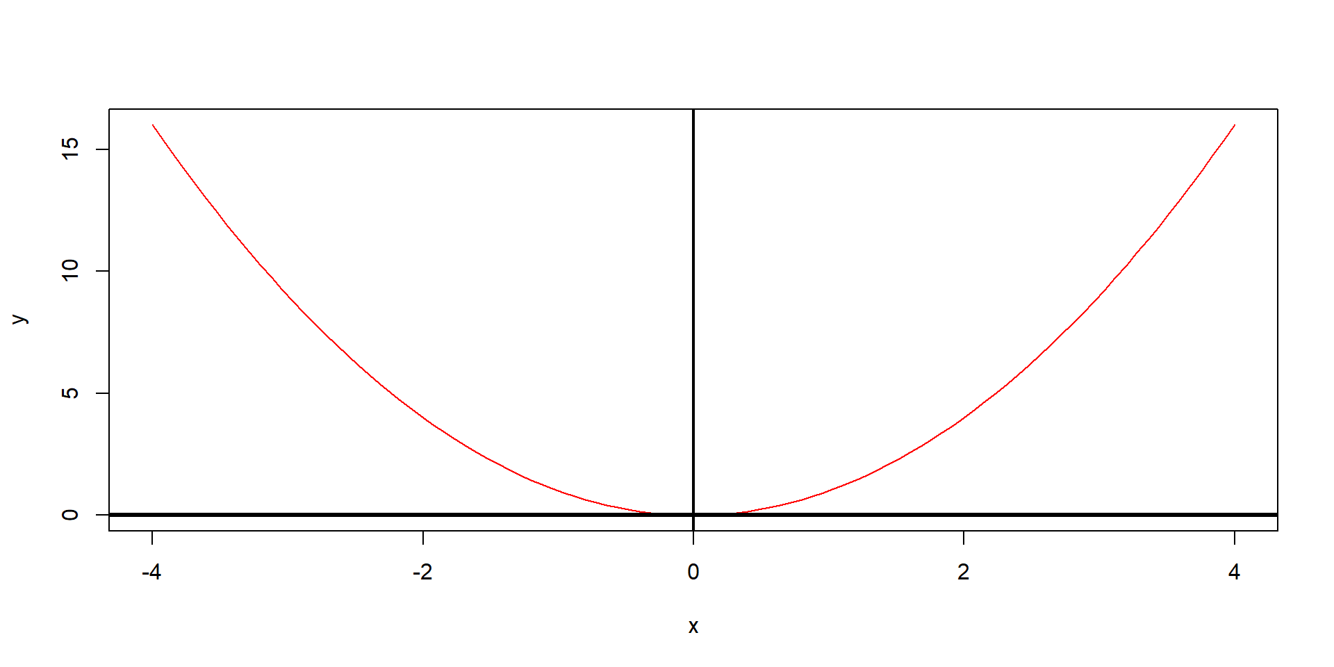
- graph of \(y = x^2\)
2.3.4 Factoring
- Factoring is a process to represent an expression in smaller multiplicative blocks.
- Example:
\[ 9x-5x^2+11x+15x^2+x^3\]
- In this case we combine all the terms that have the same exponent, which gives us \(x^3+9x^2+20x\) then we decompose the expression into smaller pieces (factors).
\[x(x+5)(x+4)\]
2.3.4.1 Factoring Quadratic Polynomials
Quadratic polynomials functions where the highest power is of order 2:\(x^2, x^2-4, x^2-2x+3\), or \(7-12x+6x^2\). Quadratic polynomials can be factored into the product of two terms: \((x \pm ?) \times (x \pm ?)\) where you need to determine whether the sign is \(+\) or \(-\), and then replace the question marks with the proper values.
for quadratic polynomials structured as \(ax^2+bx+c\) we can use the quadratic formula to get the factors.
\[\frac{-b\pm \sqrt{b^2-4ac}}{2a} \]
2.3.4.2 Factoring and Fractions
Consider the fraction \(\frac{x^2-1}{x-1}\)
We can factor the numerator \(x^2-1=(x+1)(x-1)\). We can thus rewrite the fraction as follows:
\[\frac{x^2-1}{x-1}=\frac{(x+1)(x-1)}{x-1}\]
The term \(x-1\) is in both the numerator and the denominator and thus (as long as \(x\neq 1\)) cancels out, leaving \(x+1\) for \(x \neq 1\)
2.3.5 Expansion: The FOIL Method
\[(a + b)^2 \]
\[=(a + b)(a + b)\]
\[=a^2 + 2ab + a^2\]
Example: \((2x+7) (4+3x)\)
F: Multiply the first terms: \((\underline{2x}+7) (\underline{4}+3x)=2 x \times 4=8 x\)
O: Multiply the outer terms: \((\underline{2x}+7) (4+\underline{3x})=2 x \times 3 x=6 x^2\)
I: Multiply the inner terms: \((2x+\underline{7}) (\underline{4}+3x)=4 \times 7=28\)
L: Multiply the last terms: \((2x+\underline{7}) (4+\underline{3x})=7 \times 3x=21 x\)
Add terms to get: \(8x+6x^2+28+21x\)
Finally, group like terms to get: \(6x^2+29x+28\)
To test yourself, factor the final expression and show it yields the simplified expression with which we started. This is one way to check your work for any mistakes.
2.3.5.1 Solving Quadratics
The general form of a quadratic equation:
\[
ax^2+bx+c=0
\]
The general solutions to this equation: \[ x=\frac{-b \pm \sqrt{b^2-4ac}}{2a} \]
2.3.6 Logarithms (Properties of log)
- Logarithms: \(log_a x\)
- \(a^{log_a x}=x\)
- \(log_a a^x=x\)
- if \(log_a x=b\), then \(a^{log_ax}=a^b\), thus \(x=a^b\)
- The base for the natural log is the \(e \approx 2.7183\)
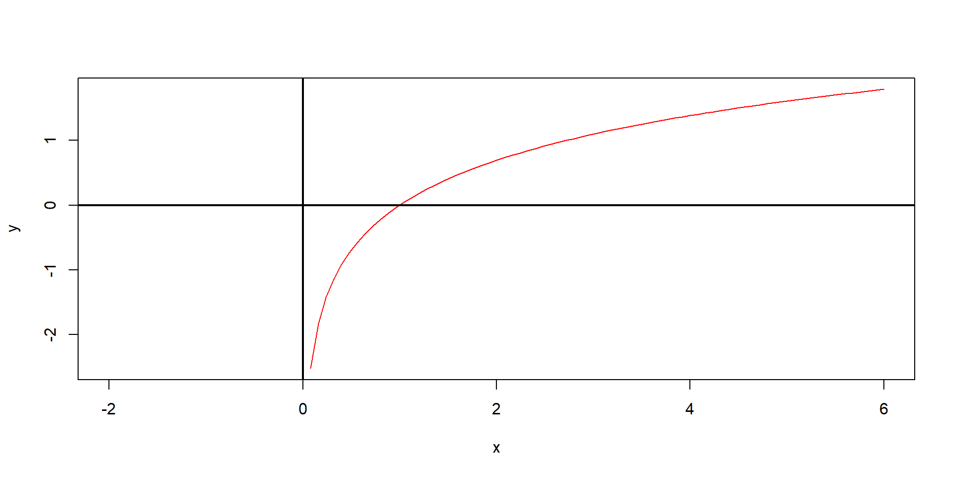
- graph of \(\ln(x)\)
Example:
If you suspect that education increases the probability of voting in national elections, but that each additional year of education has a smaller impact on the probability of voting than the preceding year’s, then the log functions are good candidates to represent that conjecture.
if \(p_v\) is “probability of voting” and \(ed\) is “years of education”:
- then \(p_v= \alpha + \beta ed\) specifies a linear relationship where an additional year of education has the same impact on the probability of voting regardless of how many years of education one has had.
- \(p_v= \alpha + \beta ed^2\) represents the claim that the impact of education on the probability of voting rises the more educated one becomes.
- We transform the relationship between \(p_v\) and \(ed\) from a linear one to a nonlinear one where the impact of an additional year of education declines the more educated one becomes: \(p_v= \alpha + \beta (\ln(ed))\)
- Algebraic rules for logs
\[\ln(x_1 \cdot x_2)=\ln(x_1)+\ln(x_2) \text{, for }x_1,x_2>0\]
\[\ln \frac{x_1}{x_2}=\ln(x_1)-\ln(x_2) \text{, for }x_1,x_2>0\]
\[\ln(x_1 + x_2) \neq \ln(x_1)+\ln(l_2) \text{, for }x_1,x_2>0\]
\[\ln(x_1 - x_2) \neq \ln(x_1)-\ln(lx) \text{, for }x_1,x_2>0\]
\[\ln(x^b)=b\ln(x) \text{, for } x>0\]
\[\ln(1+x) \approx x \text{, for } x>0 \text{ and } x \approx 0\]
2.3.7 exponentials
- exponential functions take the form of \(a^x\) where \(a\) is a constant.
- unlike log exponential functions increase at an increasing rate so they are bowed downward. exponential functions are also the inverse of logarithmic functions, so \(log_a(x)\) inverse is \(a^x\).
- the most commonly used exponential function is \(e^x\) or the inverse of natural log. The reason is that the constant e is powerful comes from the 2 places where it is derived from.
- in the equation \(a_n = (1+\frac{1}{n})^n\) if you put \(n \rightarrow \infty\) then \(a_n \rightarrow e\).
- similarly if you sum up the sequence of \(\frac{1}{n!}\) as \(n\rightarrow \infty\) we get e.
- the first result represents compound interest and the second is a power series representing individual contributions over time and is extremely useful in statistics.
2.3.8 Inequalities
- All pairs of real numbers have exactly one of the following relations: \(x=y\), \(x>y\), or \(x<y\).
- Adding any number to each side of these relations will not change them; this includes the inequalities.
That is, inequalities have the same addition and subtraction properties as equalities such that: if \(x>y\), then \(x+a>y+a\) and \(x-a>y-a\)
- You flip the \(<\) or \(>\) sign when multiplying or dividing by a negative. Multiplying or dividing an inequality by zero is not allowed.
- For multiplication, if \(a\) is positive and \(x>y\), then \(ax>ay\).
If \(a\) is negative and \(x>y\), then \(ax<ay\). - For division, if \(a\) is positive and \(x>y\), then \(\frac{x}{a}>\frac{y}{a}\).
If \(a\) is negative and \(x>y\), then \(\frac{x}{a}<\frac{y}{a}\).
Example:
Solve for \(y\):
\[-4y>2x+12\]
\[ y<-\frac{x}{2}-3 \]
Inverse Functions Example
Inverse function If $f(x) = 2x + 3 $
Put y in place of f(x) $ y = 2x + 3 $
Switch x and y $ x = 2y + 3 $
solve for y
\[ y = \frac{x - 3}{2} \]
replace y with \(f^{-1}(y)\), such that
$$
    f^{-1}(y) = \frac{x - 3}{2}
$$- \[ f(f^{-1}(x)) = f(\frac{x - 3}{2}) = x \]
- \[ f^{-1}(f(x)) = f^{-1}(f(2x + 3)) = x \]
2.4 Systems of equations
- many times we are given multiple variables to identify and equations relating them. These are called systems of equations. we assume the numbers a,b,c are know and we want answers for x and y \[ c_1 = a_1x+b_1y\\ c_2 = a_2x+b_2y\]
- in order to get a single answer for our variables one thing must hold true: there must be as many equations as there are variables. this is called just identification, if there are less equations then variables we are under identified and have an infinite amount of possibilities. if we have too many equations, then we are over identified and one is either repetitive or we might have no solution.
- there are two main ways to solve systmes of equations: substitution and elimination
2.4.1 substiution
- when given our system of equations \[ c_1 = a_1x+b_1y\\ c_2 = a_2x+b_2y\]
- we can solve this by solving one equation for one variable and plugging it into the other equation.
- first we solve equation 1 for x so \[x = \frac{c_1 - b_1y}{a_1} \]
- then we substitute our solution for x into equation 2 \[ c_2 = a_2(\frac{c_1 - b_1y}{a_1})+b_2y\]
- we then simplify and combine like terms \[ c_2 -\frac{a_2c_1}{a_1} = (\frac{a_2b_1}{a_1}+b_2)y \]
- from here we can then get an expression for y and substitute it back into our expression for x. \[ y = \frac{c_2 -\frac{a_2c_1}{a_1}}{\frac{a_2b_1}{a_1}+b_2}, x = \frac{c_1 - b_1y}{a_1}\]
2.4.2 elimination
- given our system of equations we can so something where we subtract/add one from the other after making the two coefficients on one of our variables the same to eliminate them and get an equation with one variable and a constant.
\[ c_1 = a_1x+b_1y\\ c_2 = a_2x+b_2y\]
- we make the coefficient on x equal in both cases by multiplying both equations by the others coefficient \[ a_2(c_1 = a_1x+b_1y)\\ a_1(c_2 = a_2x+b_2y)\]
- this gives \[ a_2c_1 = a_2a_1x+a_2b_1y\\ a_1c_2 = a_1a_2x+a_1b_2y\]
- we can then subtract equation 2 from equation 1 \[ a_2c_1 = a_2a_1x+a_2b_1y\\ -(a_1c_2 = a_1a_2x+a_1b_2y) \] \[ a_2c_1-a_1c_2 = (a_2b_1-a_1b_2)y\]
- we can then simplify plug back into the equation and get the same answer as we got from substitution.
Exercise 2 and Break:
solving and simplifying
problem 1
Solve for x:$1.4x^2+3.7x+1.1=0 $
problem 2
Simplify this expression as much as possible: \(\frac{2x^2 + 20x + 50}{2x^2 - 50}\)
problem 3
FOIL: \((2x - 3)(5x + 7)\)
problem 4
Complete the square and solve for y: \(\frac{1}{3}y^2 + \frac{2}{3}y - 16 = 0\)
problem 5
Solve $ > $
Problem 6
Simplify \(\frac{x^3}{x^{-3}}\).
Problem 7
Show that \(x^{m/n} = \sqrt[n]{x^m} = (\sqrt[n]{x})^m\).
Problem 8
Simplify \(h(x) = g(f(x))\), where \(f(x) = x^2 + 2\) and \(g(x) = px - 4\).
Problem 9
Simplify \(h(x) = f(g(x))\) with the same \(f\) and \(g\). Is it the same as your previous answer?
3.1 Trigonometry
- there are two main uses in social science modeling for trigonometry: modeling waves or cyclic behavior, and change of base.
- trigonometry is based on the Pythagorean Theorem that for any right triangle with sides A,B,C and C is the longest \(A^2+B^2 = C^2\)
- if we have angles a,b,c which stand opposed to A,B,C in a right triangle,
taking \(\sin(a)\) translates to \(\frac{A}{C}\)
taking \(\cos(a)\) translates to \(\frac{B}{C}\)
taking \(\tan(a)\) translates to \(\frac{A}{B}\)
- an important result is that \(cos^2(x)+sin^2(x)=1\), this is just the Pythagorean Theorem rewritten relative to an angle.
3.1.1 waves
- if we look at the graphs of theses functions we notice that the \(\sin(x), \cos(x)\) functions are waves. This is especially useful because if we want to model a cyclic behavior we have a function ready to go as a base of our analysis.
- the main difference in which function we use comes from our desired y intercept, if we want the y intercept to start at the center of our wave (0 in a standard wave) then we use \(\sin(x)\) whereas if we want it away from the center we use \(\cos(x)\).
- to change the strength of the oscillation we just add a coefficient \(\lambda\) to the front of our function and to change the frequency we can multiply x by \(\delta\) so \(\lambda\sin(\delta x)\). naturally we can make this \(\lambda\) a function of x itself so as x progresses the coefficient can vary over time in some meaningful way, for example \(\sqrt(x)\sin(x)\) has increasing magnitude while \(e^{-{x}}\sin(x)\) has decreasing magnitude.
3.1.2 change of base
- one very useful tool of trigonometry is being able to go from Cartesian (rectangular) coordinates to polar (circular) coordinates.
- polar coordinates are a different type of coordinate system to represent the same point in 2 dimensional space. A polar coordinate contains an angle and a distance to the origin or central point (pole). We then take go from the Pole representing a 0 distance and assign a certain line the quality of being 0 degrees (typically the x axis).
- angles can be represented 2 ways: degrees and radians. in a circle there are 360 degrees or \(2\pi\) radians. When the angel gets larger we are moving in a counterclockwise rotation, if we started with angle 0 being the positive x axis then 90 degrees is the positive y axis and so on.
- similarly to how we have a line in rectangular space we have a circle around the origin in polar space.
there are also spherical or cylindrical coordinates if you are doing something in 3 dimensions.
- the ability to transition between these two is based on the Pythagorean theorem. In rectangular coordinates this looks like \(x^2+y^2 = r^2\) where x and y correspond to the respective point and r is the distance (radius) from the origin. We can then use \(\arctan(\frac{y}{x})\) (inverse of tangent) to get the angle.
- going from polar to rectangular where we are given an angle \(\theta\) and a radius or magnitude r what we do is use the relationships between \(\sin(\theta)= \frac{x}{r}, \cos(\theta)= \frac{y}{r}\) to solve for x and y, giving us \(x = r\sin(\theta), y = r\cos(\theta)\)
- why do we care?
- sometimes it is simpler for us to describe behaviors through a change in direction and the magnitude, in other words a shift in position and intensity. for example in a voter model we might model our political spectrum as a continuum where the angle represents the position on the political spectrum and the radius the strength of those beliefs.
3.2 Sequences and Series
3.2.1 Sequences
Sequences are patterned sets of numbers for example {1,2,3…}, {2,4,6…}, {1,4,9,16…}, {1,3,5,7,11…} these are what is called discrete or non continuous.
most data we collect is in a discrete form with a certain frequency (weekly, monthly, quarterly annually) which means it has an observation date that is evenly spaced out.
- since these are patterned we can sometimes find formulas to represent them with the first one we know that is just \(n+1\) the second one \(n+1\), the third \(n^2\), what about the last one?
- for us the important things here are convergence and oscillation.
3.2.1.1 convergence
- a sequence \(a_n\) converges if for all N \(\lim_{n\rightarrow N} a_n \rightarrow L\) where L is a finite number. It is especially prudent for our cases when \(N = \infty\). if it goes to infinity then it is divergent.
to prove that a sequence converges the two main rules are find the functional form and take a limit as the function approaches infinity, or for sequences that do not have a well defined functional form use what is called the sandwich theorem, which is find two well defined sequences \(b_n, c_n\) this sequence exists between, \(b_n<a_n<c_n\) and see if these are bounded.
3.2.1.2 oscillation
- similar to the trigonometric equations we can use sequences to model oscillation the main way this is done is by adding a \((-1)^n\) in front of a function.
- for example: \((-1)^n n^2\) or \((-1)^n \ln(n)\)
- looking at the first term \((-1)^n\), we know that for any even n this will be 1 and any odd n \(-1\) we can change this by making it n+1, importantly this allows us to model discrete time varying data.
- lets talk about auto regressive.
3.2.2 series
- a series is a summation of a sequence represented by \(\sum_{n}(a_n)\) this is also called an accumulation. Summation similarly to sequences has convergence or divergence.
- in social sciences series are important for understanding phenomena such as accumulated wealth, or assets, or price levels, or total amount of people who have been incarcerated/arrested.
- the most important thing to remember when dealing with series is that in order for a series to converge the sequence it is taken over converges to 0 however that does not guarantee that a series will converge.
- does the series \(\sum_{n=1}^\infty {\frac{1}{n}}\) converge?
- series in this form are called p where p refers to the exponent on n. if p is greater than 1 then it converges if it is less than or equal to 1 then the series diverges, even though the sequence has converges to 0.
- how about \(\sum_{n=0}^\infty {.9^n}\) and \(\sum_{n=0}^\infty {(-1)^n}\)?
- the first converges however the second does not these are geometric series if a geometric series converges it converges to \(\frac{a}{1-r}\) where a is the first term so 1 in our case and r is the decimal so .9
Any Questions?
